This guide builds a complete Grafana dashboard for a Nokia SR OS node from gNMIc telemetry: interface throughput, packet rates, CPU and memory, BGP peers and ISIS adjacencies.

Assumptions

• gNMIc is already streaming from SR OS and exposing metrics on port 9804 with a specific prefix

• Prometheus is scraping gNMIc

• Grafana runs at http://:3000

• Basic knowledge of PromQL

Part 1: Confirm the data exists

Dashboards fail because the metric names are wrong, not because of styling. This initial step is very important.

1.1 Check gNMIc is exposing the metrics

curl -s localhost:9804/metrics | grep '^sros_' | head -20

# Output sample 

sros_state_port_statistics_in_octets{port_port_id="1/1/c1",source="172.20.20.20",subscription_name="port_stats_nokia"} 0 1791161161504
sros_state_port_statistics_in_octets{port_port_id="1/1/c1/1",source="172.20.20.20",subscription_name="port_stats_nokia"} 8.224912605e+09 1791161161504
sros_state_port_statistics_in_octets{port_port_id="1/1/c1/2",source="172.20.20.20",subscription_name="port_stats_nokia"} 0 1791161161504
sros_state_port_statistics_in_octets{port_port_id="1/1/c1/3",source="172.20.20.20",subscription_name="port_stats_nokia"} 0 1791161161504
sros_state_port_statistics_in_octets{port_port_id="1/1/c1/4",source="172.20.20.20",subscription_name="port_stats_nokia"} 0 1791161161504
sros_state_port_statistics_in_octets{port_port_id="1/1/c2",source="172.20.20.20",subscription_name="port_stats_nokia"} 0 1791161161504
sros_state_port_statistics_in_octets{port_port_id="1/1/c2/1",source="172.20.20.20",subscription_name="port_stats_nokia"} 0 1791161161504

If this is empty, stop. The problem is in gNMIc or on the router, not Grafana.

1.2 List the unique metric names

curl -s localhost:9804/metrics | grep '^sros_' | cut -d'{' -f1 | sort -u

Typical names:

sros_state_port_statistics_in_octets
sros_state_port_statistics_in_packets
sros_state_port_statistics_out_octets
sros_state_port_statistics_out_packets
sros_state_router_bgp_neighbor_statistics_session_state
sros_state_router_isis_interface_adjacency_oper_state

1.3 Look at the labels in one series

curl -s localhost:9804/metrics | grep 'in_octets' | head -3

Example :

sros_state_port_statistics_in_octets{port_port_id="1/1/c1",source="172.20.20.20",subscription_name="port_stats_nokia"}

• gNMIc builds a label name from the path element plus the key name, so port[port-id=*] becomes port_port_id

• source is the target address exactly as written in the gNMIc config

The label names you see (port_port_id, source) are what you filter and group by.

1.4 Confirm Prometheus is scraping

Open http://:9090/targets. The gNMIc job must show UP. Then run sros_state_port_statistics_in_octets in the Prometheus query box. If it returns rows, Grafana will see it.

Part 2: Connect Grafana to Prometheus

1. Log in to Grafana (default admin / admin on first run).

2. Left menu: Connections, Data sources, Add new data source, Prometheus.

3. Set the fields: Name - Prometheus, URL - http://prometheus:9090 (host IP address) , Scrape Interval - 15s matching prometheus.yml

4. Click Save & test. You want a green "Successfully queried the Prometheus API" message

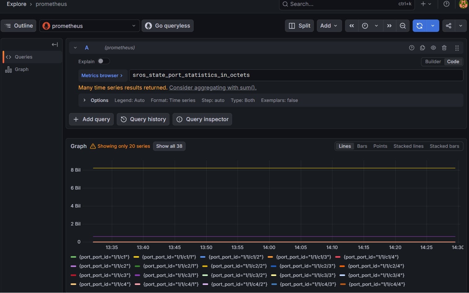
5. Test a query. Open Explore, choose the Prometheus data source, switch the editor to Code, and run:

sros_state_port_statistics_in_octets

You should see one line per port. If not, return to Part 1. Nothing later works until this does.

Part 3: Create the dashboard and variables

1. Dashboards, New, New dashboard. Do not add a panel yet.

2. Click the gear icon (Settings), open the Variables tab, then Add variable.

Variable 1: node

Field	Value
Variable Type	Classic query
Name	node
Label	Node
Data source	Prometheus
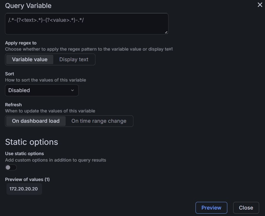
Query	label_values(sros_state_port_statistics_in_octets, source)
Multi-value	On
Include All option	On

Click Preview. You should see a router IP; in my example, it is 172.20.20.20. Click Back to list.

Variable 2: port

Field	Value
Variable Type	Classic Query
Name	port
Label	Port
Query	label_values(sros_state_port_statistics_in_octets{source=~"$node"}, port_port_id)
Multi-value	On
Include All option	On

The {source=~"$node"} filter makes the port list depend on the selected node.

Click Back to dashboard, save, and give it a name. Two dropdowns now appear at the top. Every panel below uses them.

Part 4: Panel 1, Interface throughput

1. Add, Visualization, select the Prometheus data source, and choose Time series.

2. Switch the query editor from Builder to Code.

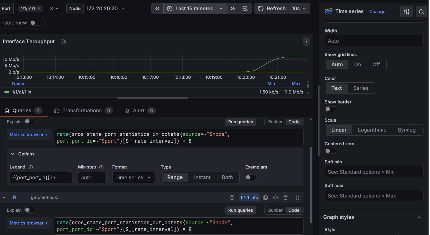
Query A (inbound) , legend {{ port_port_id }} in :

rate(sros_state_port_statistics_in_octets{source=~"$node",
port_port_id=~"$port"}[$__rate_interval]) * 8

Query B (outbound , click + Query) , legend {{ port_port_id }} out :

rate(sros_state_port_statistics_out_octets{source=~"$node",
port_port_id=~"$port"}[$__rate_interval]) * 8

Why each part exists:

• rate(...[$__rate_interval]) turns a constantly growing counter into a per-second rate.

• * 8 converts bytes to bits, which is how link speeds are quoted.

• $node and $port come from the dropdowns.

Panel Options

• Title: Interface Throughput.

• Standard options, Unit: Data rate, bits/sec (SI). Type unit in the options search box to jump to it.

• Legend, Mode: Table; Values: Mean and Max

Part 5: Panel 2, Packet rate

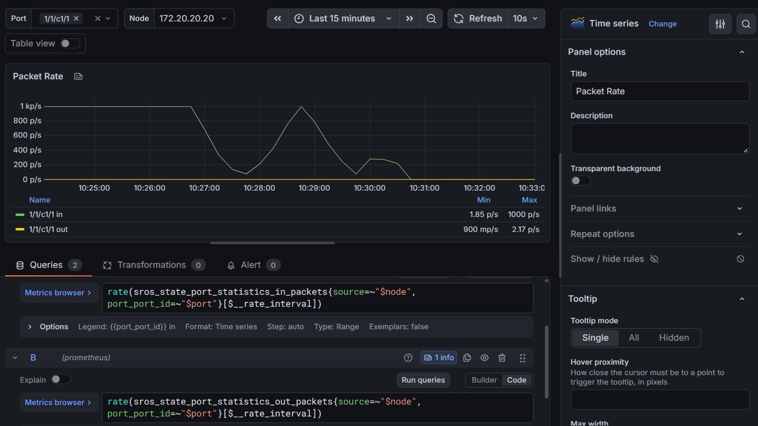
Duplicate Panel 1: panel menu, More, Duplicate. Edit the copy.

Query A (inbound) , legend {{ port_port_id }} in :

rate(sros_state_port_statistics_in_packets{source=~"$node", port_port_id=~"$port"}[$__rate_interval])

Query B (outbound , click + Query) , legend {{ port_port_id }} out :

rate(sros_state_port_statistics_out_packets{source=~"$node", port_port_id=~"$port"}[$__rate_interval]) 

There is no * 8 here, since packets are not bytes. Title: Packet Rate. Unit: Throughput, packets/sec.

Part 6: Panel 4, CPU and memory

Find the exact leaf names from your system_resources subscription:

# Execute 

curl -s localhost:9804/metrics | grep -Ei 'cpu|memory' | cut -d'{' -f1 | sort -u

# Output 
sros_state_system_cpu_summary_busiest_core_utilization_cpu_time
sros_state_system_cpu_summary_busiest_core_utilization_cpu_usage
sros_state_system_cpu_summary_busiest_core_utilization_time_used
sros_state_system_cpu_summary_idle_cpu_time
sros_state_system_cpu_summary_idle_cpu_usage
sros_state_system_cpu_summary_idle_time_used
sros_state_system_cpu_summary_total_cpu_time
sros_state_system_cpu_summary_total_cpu_usage
sros_state_system_cpu_summary_total_time_used
sros_state_system_cpu_summary_usage_cpu_time
sros_state_system_cpu_summary_usage_cpu_usage
sros_state_system_cpu_summary_usage_time_used
sros_state_system_memory_pools_summary_available_memory
sros_state_system_memory_pools_summary_current_total_size
sros_state_system_memory_pools_summary_total_in_use

CPU gauge

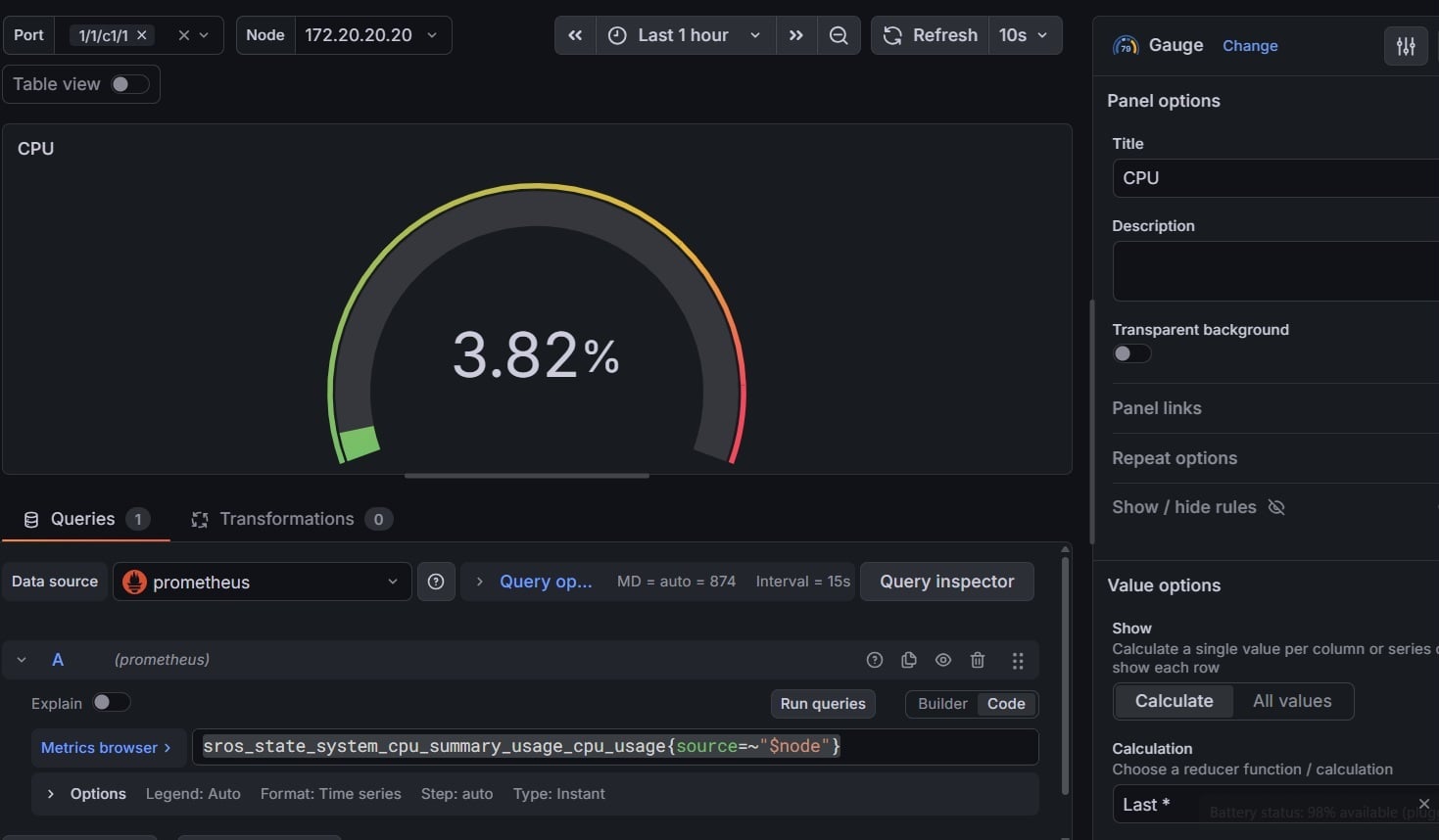
1. Add, Visualization, Gauge.

2. Query:

   sros_state_system_cpu_summary_usage_cpu_usage{source=~"$node"}
   

3. Unit: Percent (0-100). Min: 0. Max: 100.

4. Thresholds: base green, 70 amber, 90 red.

5. Title: CPU.

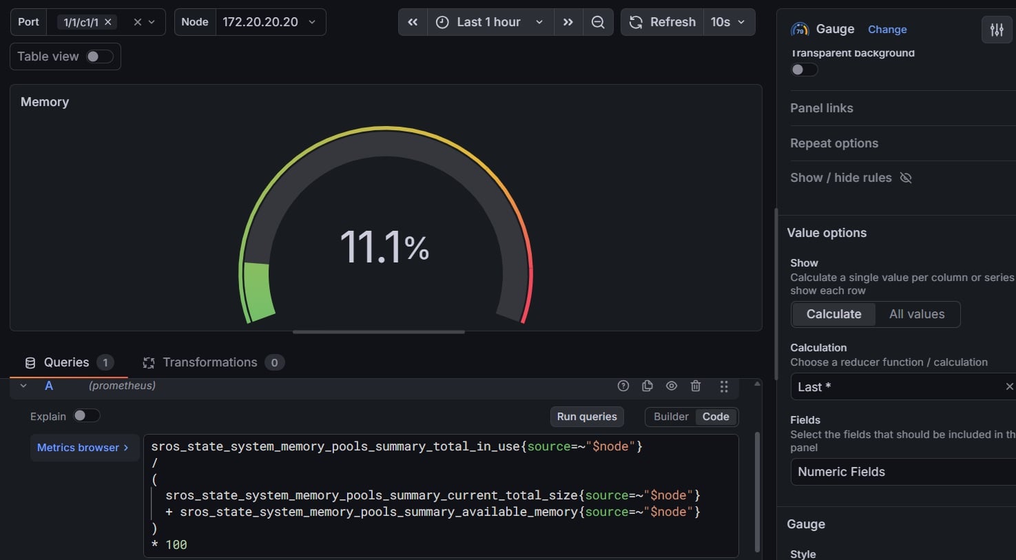
Memory: plot it the same way. If you only have allocated and available bytes, compute it:

Query:

sros_state_system_memory_pools_summary_total_in_use{source=~"$node"}
/
(
  sros_state_system_memory_pools_summary_current_total_size{source=~"$node"}
  + sros_state_system_memory_pools_summary_available_memory{source=~"$node"}
)
* 100

Part 7: Panel 5, BGP peers

Stat: BGP peers established

1. Add, Visualization, Stat.

2. Query:

   sum(sros_state_router_bgp_neighbor_statistics_session_state{source=~"$node"})
   

3. Title: BGP Peers Established

4. Thresholds: base red, 1 green (or your expected peer count).

5. Color mode: Background.

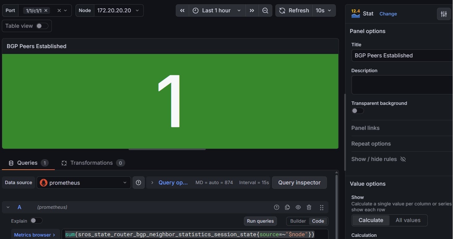
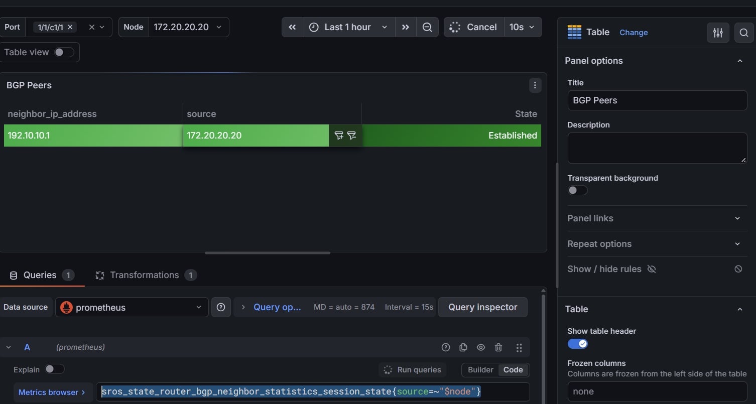
Table: per-peer state

1. Add, Visualization, Table

2. Query:

   sros_state_router_bgp_neighbor_statistics_session_state{source=~"$node"}
   

3. Transform, Organize fields by name: hide Time, name, app, job, instance, subscription_name; rename Value to State.

4. Value mappings: 1 to Established (green), 0 to Down (red).

5. Cell options, Cell type: Colored background.

Part 8: Panel 6, ISIS adjacencies

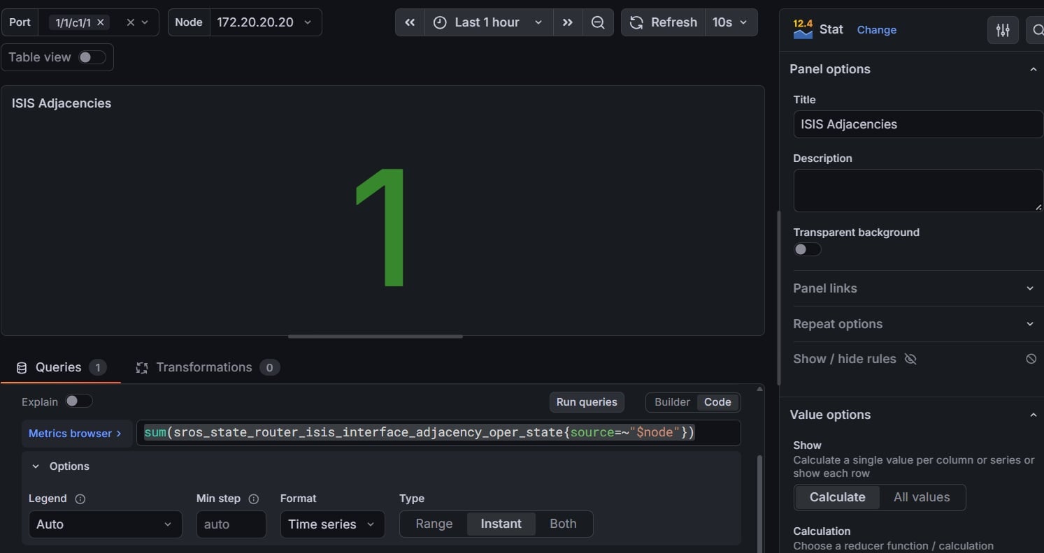
Stat

1. Add, Visualization, State timeline.

2. Query:

   sum(sros_state_router_isis_interface_adjacency_oper_state{source=~"$node"})
   

3. Thresholds: red base, green at your expected adjacency count.

4. Title: ISIS Adjacencies

Part 9: Arrange the layout

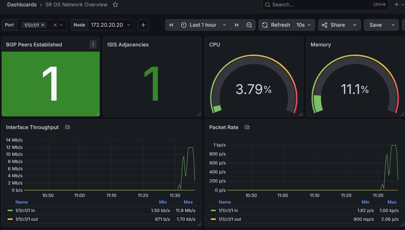
Row	Panels
Top	BGP Peers Established, ISIS Adjacencies Up, CPU gauge, memory gauge
Middle	Interface Throughput (wide), Packet Rate

Part 10: Finishing touches

1. Top right: Time range Last 1 hour; Refresh 10s.

2. Save with Ctrl+S and add a version note.

3. Export the dashboard: Export, Export as JSON, tick Export for sharing externally, Save to file. The data source becomes a variable, so the JSON imports cleanly into any other Grafana or into Git.

Part 11: Troubleshooting a blank panel

1. Run the query in Explore. If Explore is empty, the problem is the query or the data, not the panel.

2. Remove label filters. Delete {source=~"$node", port_port_id=~"$port"} and retry. If data appears, a label name or variable value is wrong.

3. Check spelling against /metrics. port_port_id versus port-id is the classic mistake.

4. Widen the time range. on_change series can look empty over a very short window.

5. Rates show "No data". rate() needs at least two samples inside the window, so $__rate_interval should be at least four times the scrape interval.